
1. Linear regression
This term stands for a process of statistical analysis to test the relationship between two continuous variables, the first is independent and the second is one dependent
This type of statistics is used to find the best line through a set of data points that in turn will reveal the best future predictions
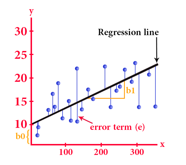
The simple linear regression equation is as follows:
y = b0 + b1*x
y is the dependent variable
x represents the independent variable
b0 represents the y-intercept (the point of intersection of the y-axis with the line)
b1 represents the slope of the line
And by the method of least squares, we can get the most appropriate line, that is, the line that reduces the sum of the square differences between the actual and expected values of the value of y
We can also customize the work of linear regression to expand it to several independent variables, then it is called multiple linear regression, whose equation is as follows:
y = b0 + b1x1 + b2x2 +… + bn * xn
x1, x2, …, xn represent the independent variables
b1, b2, …, bn represent the corresponding variables
As mentioned above, linear regression is useful for obtaining future predictions, as is the case when predicting stock prices or determining future sales of a specific product, and this is done by making predictions about the dependent variable
However, there are cases in which the regression model is not very accurate, in the event that there are extreme values that do not take the direction of the data in general
In order to show the optimal treatment in linear regression in the presence of extreme values, the following figure is given
– Neutralizing outliers from the data set before training the model
– Minimize the effect of outliers by applying a transform as taking a data log
Use powerful regression methods such as RANSAC or Theil-Sen because they mitigate the negative impact of outliers more effectively than traditional linear regression.
However, it cannot be denied that linear regression is an effective and commonly used statistical method
2. Logistic regression
It is a statistical method used to obtain predictions for options that bear two options, i.e. binary outcome, by relying on one or more independent variables, and this regression has a role in classification and sorting functions, such as predicting customer behavior and other tasks.
The work of logistic regression is based on a sigmoid function that sets the input variables to a probability between 0 and 1, and then comes the role of the prediction to get the possible outcome
Logistic regression is represented by the following equation:
P(y=1|x) = 1/(1+e^-(b0 + b1x1 + b2x2 + … + bn*xn))
P(y = 1|x) represents the probability that the outcome of y is 1 compared to the input variables x
b0 represents the intercept
b1, b2, …, bn represent the coefficients of the input variables x1, x2, …, xn
By training the model on a data set and using the optimization algorithm, the coefficients are determined and then used to make predictions by entering new data and calculating the probability that the result is 1
In the following diagram we see the logistic regression model
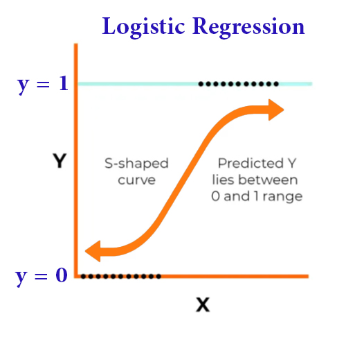
By examining the previous diagram , we find that the input variables x1 and x2 were used to predict the result y that has two options.
This regression is tasked with assigning the input variables to a probability that will determine in the future the shape of the expectation of the outcome
The coefficients b1 and b2 are determined by training the model on a data set and setting the threshold to 0.5.
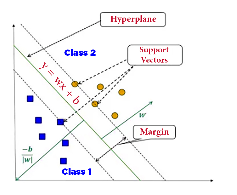
3. Support Vector Machines (SVMs)
SVM is a powerful algorithm for both classification and regression. It divides data points into different categories by finding the optimal level with maximum margin. SVMs have been successfully applied in various fields, including image recognition, text classification, and bioinformatics.

The cases where SVMs are used are when the data cannot be separated by a straight line, this channel can distribute the data over a high-dimensional swath to facilitate the detection of nonlinear boundaries
SVMs have proven memory utilization, they focus on storing only the support vectors without the entire data set, and they are highly efficient in high-dimensional spaces even if the number of features is greater than the number of samples
This technique is strong against outliers due to its dependence on support vectors
However, one of the drawbacks of this technique is that it is sensitive to kernel function selection, and it is not effective for large data sets, as its training time is often very long.
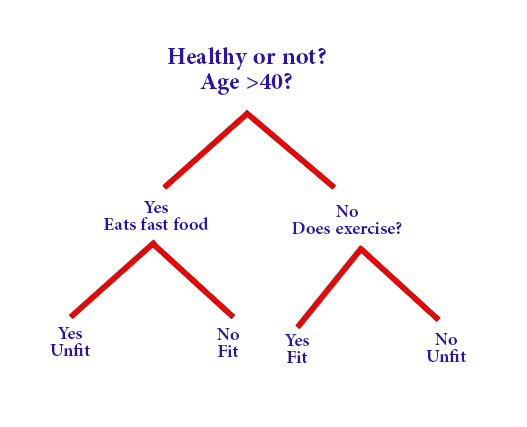
4. Decision Trees:
Decision trees are multi-pronged algorithms that build a tree-like model of decisions and their possible outcomes. By asking a series of questions, decision trees classify data into categories or predict continuous values. They are common in areas such as finance, customer segmentation, and manufacturing
So, it is a tree-like diagram, where each internal set forms a decision point, while the leaf node expresses prediction
To explain how the decision tree works:
The process of building the tree begins with selecting the root node so that it is easy to sort the data into different categories, then the data is iteratively divided into subgroups based on the values of the input features in order to find a classification formula that facilitates the sorting of the different data or required values
The decision tree diagram is easy to understand as it enables the user to create a well-defined visualization that allows the correct and beneficial decision-making

However, it should be known that the deeper the decision tree and the greater the number of its leaves, the greater the probability of neglecting the data, and this is one of the negative aspects of the decision tree.
If we want to talk about other negative aspects, it must be noted that the decision tree is often sensitive to the order of the input features, and this leads to different tree diagrams, and on the other hand, the final tree may not give the best result.
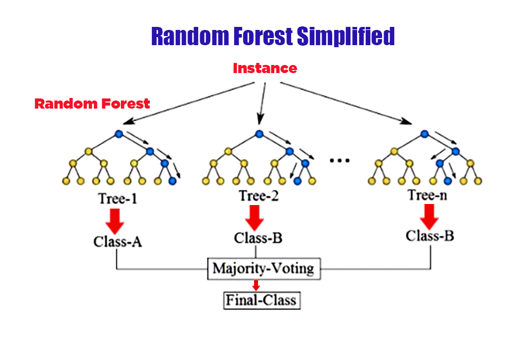
5. Random Forest:
The random forest is a group learning method that combines many decision trees to improve prediction accuracy. Each tree is built on a random subset of the training data and features. Random forests are effective for classification and regression tasks, finding applications in areas such as finance, healthcare, and bioinformatics.
Random forests are used if the data in a single decision tree is subject to overfitting, thus improving the model with greater accuracy

This forest is formed using the Bootstrapping technique which generates multiple decision trees
It is a statistical method based on randomly selecting data points and replacing them with the original data set. As a result, multiple data sets are formed that include a different set of data points that are later used to train individual decision trees.
Random forest allows to improve overall model performance by reducing the correlation between trees within a random forest because it relies on using a random subset of features for each tree and this method is called “random subspace”.
One of the drawbacks of a random forest is the higher computational cost of training and predictions as the number of trees in a forest increases
In addition to its lower interpretability compared to a single decision tree, it is superior to a single decision tree by being less prone to overfitting and having a higher ability to handle high-dimensional datasets.
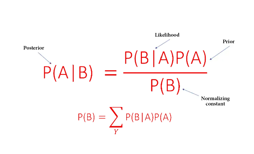
6. Naive Bayes
Naive Bayes is a probability algorithm based on Bayes’ theory with the assumption of independence between features. Despite its simplicity, Naive Bayes performs well in many real-world applications, such as spam filtering, sentiment analysis, and document classification.

Based on Bayes’ theorem, the probability of a particular class is calculated according to the values of the input features
There are different types of probability distributions when implementing the Naive Bayes algorithm, depending on the type of data
Among them:
Gaussian: for continuous data
Multinomial: for discrete data
Bernoulli: for binary data
Turning to the advantages of using this algorithm, we can say that it enjoys its simplicity and quality in terms of its need for less training data compared to other algorithms, and it is also characterized by the ability to deal with missing data.
But if we want to talk about the negatives, we will collide with their dependence on the assumption of independence between features, which often contradicts real-world data.
In addition, it is negatively affected by the presence of features different from the data set, so the level of performance decreases and the required efficiency decreases with it
7. KNN
KNN is a non-parametric algorithm that classifies new data points based on their proximity to the seeded examples on the training set. It is widely used in pattern recognition and recommendation systems
KNN can handle classification and regression tasks.

That is, it relies on assigning similarity to similar data points
After choosing the k value, the value closest to the prediction, the data is sorted into training and test sets to make a prediction for a new input by calculating the distance between the entry and each data point in the training set, then choosing the k nearest data points to set the prediction later using the closest set of data points
8. K-means
The working principle of this algorithm is based on the random selection of k centroids
So that k represents the number of clusters we want to create and then each data point is mapped to the cluster that was closest to the central point
So it is an algorithm that relies on grouping similar data points together and it is based on distance so that distances are calculated to assign a point to a group

This algorithm is used in many market segmentation, image compression and many other widely used applications
The downside of this algorithm is that its assumptions for data sets often do not match the real world
9. Dimensional reduction algorithms
This algorithm aims to reduce the number of features in the data set while preserving the necessary information. This technique is called “Dimensional Reduction”.

Like many dimension reduction algorithms, this algorithm makes data visualization easy and simple.
As in Principal Components Analysis (PCA)
and linear discriminant analysis (LDA)
Distributed Random Neighborhood Modulation (t-SNE)
We will come to explain each one separately
* Principal Component Analysis (PCA): It is a linear pattern of dimension reduction. Principal components can be defined as a set of correlated variables that have been orthogonally transformed into uncorrelated linear variables. Its aim is to identify patterns in the data and reduce its dimensions while preserving the necessary information.
* Linear Discrimination Analysis (LDA): is a supervised dimensionality reduction pattern used to obtain the most discriminating features of the sorting and classifying function
*t-Distributed Stochastic Neighbor Embedding (t-SNE)
It is a well-proven nonlinear dimension reduction technique for visualizing high-dimensional data in order to obtain a low-dimensional representation that prevents loss of data structure.
The downside of the dimension reduction technique is that some necessary information may be lost during the dimension reduction process
It is also necessary to know the type of data and the task to be performed in order to choose the dimension reduction technique, so the process of determining the appropriate number of dimensions to keep may be somewhat difficult.
10. Gradient boosting algorithm and AdaBoosting algorithm
They are two algorithms used in classification and regression functions and they are widely used in machine learning
The working principle of these two algorithms is based on forming an effective model by collecting several weak models
Gradient enhancement:
It depends on building a pattern in a progressive manner according to multiple stages, starting from installing a simple model on the data (such as a decision tree, for example) and then correcting the errors made by the previous models by adding additional models. Thus, each added model obtains agreement with the negative gradient of the loss function in terms of the predictions of the previous model.
In this way, the final output of the model is the result of assembling the individual models
AdaBoost:
It is an acronym for Adaptive Boosting. This algorithm is similar to its predecessor in terms of its mechanism of action by relying on creating a pattern for the forward staging method and differs from the gradient boosting algorithm by focusing on improving the performance of weak models by adjusting the weights of the training data in each iteration, i.e. it depends on the wrong training models according to the previous model. It then adjusts the weights for the erroneous models so that they have a higher probability of being selected in the next iteration until finally arriving at a model weighted for all individual models. These two algorithms are characterized by their ability to deal with wide types of numerical and categorical data, and they are also characterized by their strength in dealing with the extreme value and with data with missing values, so they are used in many practical applications
أشهر عشرة خوارزميات التعلم الآلي للعام 2024

1. الانحدار الخطي
يرمز هذا المصطلح إلى عملية تحليل إحصائي لاختبار العلاقة بين متغيرين مستمرين الأول مستقل والثاني تابع واحد
يستخدم هذا النوع من الإحصاء لإيجاد الخط الأفضل عن طريق مجموعة من نقاط البيانات التي بدورها ستكشف لنا التنبؤات المستقبلية الأفضل

:تتمثل معادلة الانحدار الخطي البسيط بالشكل التالي
y = b0 + b1*x
متغير التابع y يمثل
المتغير المستقل x يمثل
y تقاطع b0 يمثل
(مع الخط y نقطة تقاطع المحور)
ميل الخط b1 يمثل
وبطريقة المربعات الصغرى نستطيع الحصول على الخط الأنسب أي الخط الذي يقلل من مجموع الفروق المربعة بين القيم الفعلية
y والمتوقعة للقيمة
كما وأننا نستطيع تخصيص عمل الانحدار الخطي ليتوسع إلى عدة متغيرات مستقلة فيسمى عندها الانحدار الخطي المتعدد والذي تتمثل معادلته بالشكل التالي
y = b0 + b1x1 + b2x2 +… + bn * xn
المتغيرات المستقلة x1 ، x2 ، … ، xn تمثل
المتغيرات المقابلة b1 ، b2 ، … ، bn وتمثل
وكما ذكرنا آنفاً يفيد الانحدار الخطي للحصول على التنبؤات المستقبلية، كما هو الحال عند التنبؤ بأسعار الأسهم أو تحديد مبيعات مستقبلية لمنتج معين ويتم ذلك بإجراء تنبؤات حول المتغير التابع
إلا أنه يوجد حالات لا يكون فيها نموذج الانحدار دقيق جداً وذلك في حال وجود قيم متطرفة لا تأخذ اتجاه البيانات بشكل عام
ولتبيان التعامل الأمثل في الانحدار الخطي بوجود القيم المتطرفة على الشكل التالي
تحييد القيم المتطرفة وإبعادها من مجموعة البيانات قبل تدريب النموذج *
تقليل تأثير القيم المتطرفة عن طريق تطبيق تحويل كأخذ سجل البيانات *
Theil-Senأو RANSAC استخدام طرق الانحدار القوية مثل *
لأنها تخفف من التأثير السلبي للقيم المتطرفة بفعالية أكبر من الانحدار الخطي التقليدي
ومع ذلك لا يمكن إنكار أن الانحدار الخطي يعتبر طريقة إحصاء فعالة وشائعة الاستخدام
2. الانحدار اللوجستي
وهو طريقة إحصاء تستخدم للحصول على تنبؤات للخيارات التي تحتمل خيارين أي ثنائية النتيجة وذلك بالاعتماد على مغير مستقل أو أكثر كما وأن لهذا الانحدار دور في وظائف التصنيف والفرز كأن يتنبأ بسلوك العملاء وغيرها من المهام الأخرى
يعتمد عمل الانحدار اللوجستي على دالة سينية تقوم بتعيين متغيرات الإدخال
إلى احتمال بين صفر وواحد
ثم يأتي دور التوقع للحصول على النتيجة المحتملة
:يتمثل الانحدار اللوجستي بالمعادلة التالية
P(y=1|x) = 1/(1+e^-(b0 + b1x1 + b2x2 + … + bn*xn))
P (y = 1 | x) يمثل
1 هي y احتمال أن تكون نتيجة
x مقارنةً مع متغيرات الإدخال
التقاطع b0 تمثل
b1 ، b2 ، … ، bn تمثل
معامِلات متغيرات الإدخال
x1 ، x2 ، … ، xn
ومن خلال تدريب النموذج على مجموعة بيانات والاستعانة بخوارزمية التحسين يتم تحديد المعاملات ثم يتم استخدامه في إجراء التنبؤات عن طريق إدخال بيانات جديدة
1 وحساب احتمالية أن تكون النتيجة
في الشكل التالي نلاحظ نموذج الانحدار اللوجستي

وبدراسة الشكل السابق نجد أنه استُخدمت
y للتنبؤ بالنتيجة x2و x1 متغيرات الإدخال
التي تحتمل خيارين
يتولى هذا الانحدار مهمة تعيين متغيرات الإدخال إلى احتمالية والتي ستحدد مستقبلاً شكل التوقع للنتيجة
b2و b1 أما المعامِلان
فيتحددان من خلال تدريب النموذج على مجموعة بيانات
0.5 وتعيين الحد على
3. (SVMs) دعم آلات المتجهات
خوارزمية قوية لكل من التصنيف والانحدار SVM يعد
يقسم نقاط البيانات إلى فئات مختلفة من خلال إيجاد المستوى الأمثل مع الحد الأقصى للهامش
بنجاح في مجالات مختلفةSVMs تم تطبيق
بما في ذلك التعرف على الصور وتصنيف النص والمعلوماتية الحيوية
SVMs تعتبر الحالات التي تستخدم فيها
هي التي لا يمكن فيها فصل البيانات بخط مستقيم، فبإمكان هذه القنية أن توزع البيانات على رقعة عالية الأبعاد لتسهيل اكتشاف حدود غير خطية
قدرتها على استخدام الذاكرة SVMs أثبتت أجهزة
فهي تركز على تخزين متجهات الدعم فقط دون الحاجة إلى مجموعة البيانات كلها، كما وأنها تتمتع بكفاءة عالية في المساحات عالية الأبعاد حتى لو كان عدد الميزات أكبر من عدد العينات
تعتبر هذه التقنية قوية ضد القيم المتطرفة نظراً لاعتمادها على ناقلات الدعم
إلا أن أحد سلبيات هذه التقنية هو أنها
kernel حساسة لاختيار وظيفة
كما أنها غير فعالة لمجموعات البيانات الضخمة كونها وقت التدريب فيها طويل جداً على الأغلب
4. أشجار القرار
أشجار القرار هي خوارزميات متعددة الجوانب تبني نموذجًا شبيهًا بالشجرة من القرارات ونتائجها المحتملة. من خلال طرح سلسلة من الأسئلة، تصنف أشجار القرار البيانات إلى فئات أو تتنبأ بقيم مستمرة. وهي شائعة في مجالات مثل التمويل وتجزئة العملاء والتصنيع
إذاً هي مخطط يشبه الشجرة بحيث تشكل كل عدة داخلية نقطة قرار أما العقدة الورقية فتعبر عن التنبؤ
:ولشرح عمل شجرة القرار
تبدأ عملية بناء الشجرة باختيار عقدة الجذر بحيث يسهل فرز البيانات إلى فئات مختلفة، ثم يتم تقسيم البيانات إلى مجموعات فرعية بشكل متكرر بالاعتماد على قيم ميزات الإدخال بغية إيجاد صيغة تصنيفية تسهل فرز البيانات المختلفة أو القيم المطلوبة
مخطط شجرة القرار سهل الفهم فهو يمكن المستخدم من إنشاء تصور واضح المعالم يتيح اتخاذ القرار الصائب والمفيد
إلا يجب معرفة أنه كلما كانت شجرة القرار عميقة أكثر وكان عدد أوراقها أكبر كلما زاد احتمال التفريط في البيانات وهذا أحد الجوانب السلبية في شجرة القرار
وإذا أردنا التحدث عن جوانب سلبية أخرى فلابد من التنويه إلى أن شجرة القرار غالباً ما تكون حساسة لترتيب ميزات الإدخال وهذا يؤدي إلى مخططات شجرية مختلفة والمقابل قد لا تعطي الشجرة النهائية النتيجة الأفضل
5. الغابة العشوائية
الغابة العشوائية هي طريقة تعلم جماعية تجمع بين العديد من أشجار القرار لتحسين دقة التنبؤ، كل شجرة مبنية على مجموعة فرعية عشوائية من بيانات التدريب والميزات، تعتبر الغابات العشوائية فعالة في مهام التصنيف والانحدار وإيجاد تطبيقات في مجالات مثل التمويل والرعاية الصحية والمعلوماتية الحيوية
ويتم استخدام الغابات العشوائية في حال كانت البيانات في شجرة قرار واحدة معرضة للإفراط في التجهيز وبالتالي تحسين النموذج بدقة أكبر
Bootstrapping يتم تشكيل هذه الغابة باستخدام تقنية
التي تقوم بإنشاء أشجار قرارات متعددة
وهي طريقة إحصائية تعتمد على اختيار عشوائي لنقاط بيانات واستبدالها مع مجموعة البيانات الأصلية فتتشكل بالنتيجة مجموعات بيانات متعددة تتضمن مجموعة مختلفة من نقاط البيانات المستخدمة لاحقاً لتدريب أشجار القرار الفردية
تتيح الغابة العشوائية تحسين أداء النموذج بشكل عام عن طريق تقليل الارتباط بين الأشجار ضمن الغابة العشوائية لأنها تعتمد على استخدام مجموعة فرعية عشوائية من الميزات لكل شجرة وهذه الطريقة تسمى “الفضاء الجزئي العشوائي”
أحد سلبيات الغابة العشوائية يكمن في ارتفاع التكلفة الحسابية للتدريب والتنبؤات كلما زاد عدد الأشجار في الغابة علاوة على انخفاض قابلية التفسير مقارنة بشجرة قرار واحدة إلا أنها تتفوق على شجرة القرار الواحدة بكونها أقل عرضة للإفراط في التجهيز وقدرتها العالية على التعامل مع مجموعات بيانات عالية الأبعاد
6. Naive Bayes
هي خوارزمية احتمالية تعتمد على نظرية بايز مع افتراض الاستقلال بين الميزات
Naive Bayes على الرغم من بساطته فإن
يعمل بشكل جيد في العديد من تطبيقات العالم الحقيقي، مثل تصفية البريد العشوائي، وتحليل المشاعر، وتصنيف المستندات
بالاعتماد على نظرية بايز يتم حساب احتمالية فئة معينة وفق قيم ميزات الإدخال ويوجد أنواع مختلفة من التوزيعات الاحتمالية
تستخدم حسب نمط البيانات Naive Bayes عند تنفيذ خوارزمية
:نذكر منها
للبيانات المستمرة :Gaussian
للبيانات المنفصلة :Multinomial
للبيانات الثنائية :Bernoulli
وبالتطرق إلى إيجابيات استخدام هذه الخوارزمية فيمكننا القول أنها تتمتع ببساطتها وجودتها من حيث حاجتها لبيانات تدريب أقل مقارنة بالخوارزميات الأخرى وتتميز أيضاً بإمكانية التعامل مع البيانات المفقودة
أما إذا أردنا التحدث عن السلبيات فسنصطدم باعتمادها على افتراض الاستقلال بين الميزات والذي غالباً ما يتعارض مع بيانات العالم الواقعي
إضافة إلى أنها تتأثر سلباً بوجود ميزات مختلفة عن مجوعة البيانات فينخفض مستوى الأداء وتقل معها الكفاءة المطلوبة
7. KNN
هي خوارزمية غير معلمية تصنف نقاط البيانات الجديدة بناءً على قربها من الأمثلة المصنفة في مجموعة التدريب، يستخدم على نطاق واسع في التعرف على الأنماط وأنظمة التوصية
التعامل مع مهام التصنيف والانحدار KNN يمكن لـ
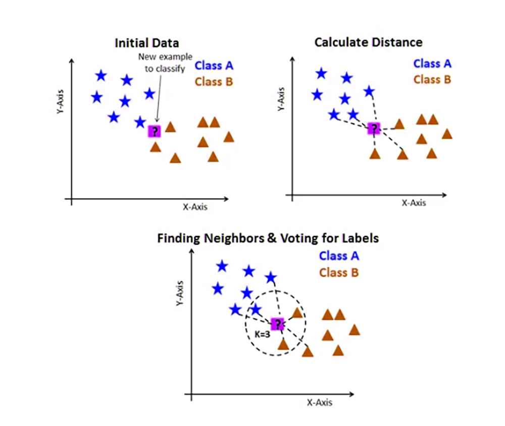
أي أنها تعتمد على إضفاء صفة التشابه على نقاط البيانات المتشابهة
القيمة الأقرب للتنبؤ k بعد اختيار قيمة
يتم فرز البيانات إلى مجموعات تدريب واختبار لعمل تنبؤ لمدخل جديد عن طريق حساب المسافة بين الإدخال وكل نقطة بيانات في مجموعة التدريب
أقرب نقاط البيانات k ثم تختار
ليتم تعيين التنبؤ لاحقاً باستخدام المجموعة الأكثر قرباً لنقاط البيانات
8. K-means
يعتمد مبدأ عمل هذه الخوارزمية
k centroids على الاختيار العشوائي لـ
عدد المجموعات التي نريد إنشاءها k بحيث تمثل
ثم يتم تحديد كل نقطة بيانات إلى المجموعة التي تم أقرب نقطة مركزية
إذاً هي خوارزمية تعتمد على تجميع نقاط البيانات المتشابهة معاً وهي قائمة على المسافة بحيث تُحسب المسافات لتعيين نقطة إلى مجموعة
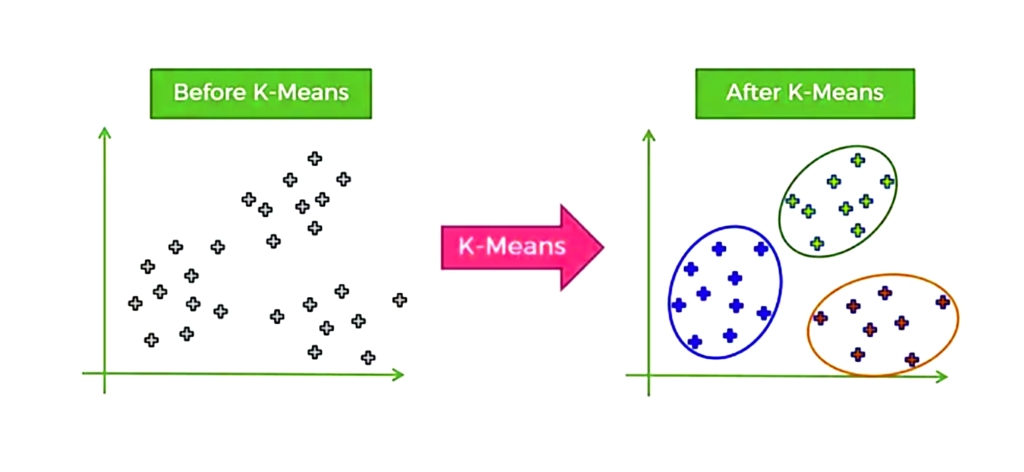
تستخدم هذه الخوارزمية في كثير من تطبيقات تجزئة السوق وضغط الصور وغيرها العديد من التطبيقات الواسعة الاستخدام
يتمثل الجانب السلبي لهذه الخوارزمية هو أن افتراضاتها لمجموعات البيانات لا تطابق الواقع الحقيقي في أغلب حيان
9. خوارزميات تقليل الأبعاد
تهدف هذه الخوارزمية إلى تقليل عدد الميزات في مجموعة البيانات مع المحافظة على المعلومات الضرورية، تسمى هذه التقنية تقليل الأبعاد
تسهم هذه الخوارزمية في جعل تصور البيانات أمراً سهلاً وبسيطاً شأنها شأن كثير من خوارزميات تقليل الأبعاد
(PCA) كما في تحليل المكونات الرئيسية
(LDA) والتحليل التمييزي الخطي
(t-SNE) والتضمين المتجاور العشوائي الموزع
وسنأتي على شرح كل واحدة منها على حدا
: (PCA) تحليل المكون الرئيسي *
هو نمط خطي لتقليل الأبعاد، ويمكن تعريف المكونات الأساسية بأنها مجموعة من المتغيرات المرتبطة تم تحويلها تحويلاً متعامداً إلى متغيرات خطية غير مترابطة، الهدف منه تحديد الأنماط في البيانات وتقليل أبعادها مع المحافظة على المعلومات الضرورية
: (LDA) تحليل التمييز الخطي *
هو نمط تقليل الأبعاد خاضع للإشراف يستخدم بغية الحصول على السمات الأكثر تمييزاً لوظيفة الفرز والتصنيف
t-Distributed Stochastic Neighbor Embedding (t-SNE) تضمين *
وهي تقنية لتقليل الأبعاد غير الخطية أثبتت جدارتها لتصور البيانات عالية الأبعاد بغية الحصول على تمثيل منخفض الأبعاد يَحُول دون فقدان بنية البيانات
تتمثل سلبيات تقنية تقليل الأبعاد هو أنه بعض المعلومات الضرورية قد تتعرض الفقدان أثناء عملية تقليل الأبعاد
كما وأنه من الضروري معرفة نوع البيانات والمهمة المطلوب تنفيذها لاختيار تقنية تقليل الأبعاد لذا قد تكون عملية تحديد العدد الأنسب للأبعاد للاحتفاظ بها صعبة نوعاً ما
10. AdaBoosting خوارزمية تعزيز التدرج وخوارزمية
وهما خوارزميتان تستخدمان في وظائف التصنيف والانحدار وهما تستخدمان على نطاق واسع في التعلم الآلي
يعتمد مبدأ عمل هاتين الخوارزميتين على تشكيل نموذج فعال من خلال جمع عدة نماذج ضعيفة
:تعزيز التدرج
تعتمد على بناء نمط بأسلوب تقدمي وفق مراحل متعددة انطلاقاً من تركيب نموذج بسيط على البيانات (كشجرة القرار مثلاً) ثم تصحيح الأخطاء التي ارتكبتها النماذج السابقة وذلك بإضافة نماذج إضافية وبذلك يحصل كل نموذج مضاف على توافق مع التدرج السلبي لوظيفة الخسارة من حيث تنبؤات النموذج السابق
وعلى هذا النحو يكون الناتج النهائي للنموذج هو حصيلة تجميع النماذج الفردية
:AdaBoost
Adaptive Boosting وهي اختصار لـ
تشبه هذه الخوارزمية سابقتها من حيث آلية عملها باعتمادها على إنشاء نمط لأسلوب المرحلي للأمام وتختلف عن خوارزمية تعزيز التدرج بتركيزها على تحسين أداء النماذج الضعيفة من خلال تعديل أوزان بيانات التدريب في كل تكرار أي أنها تعتمد على نماذج التدريب الخاطئة حسب النموذج السابق وثم تثوم بتعديل الأوزان النماذج الخاطئة بحيث يصبح لديها احتمال أكبر للاختيار في التكرار الذي يليه حتى الوصول في النهاية إلى نموذج مرجح لجميع النماذج الفردية
تمتاز هاتان الخوارزميتان إلى بقدرتهما على التعامل مع أنماط واسعة من البيانات الرقمية منها والفئوية وتمتازان أيضاً بقوتهما بالتعامل مع القيمة المتطرفة ومع البيانات ذات القيم المفقودة لذا تستخدمان في العديد من التطبيقات العملية
