


Structured Query Language (SQL) is the standard query language for relational databases. This language is simple and easy to understand, but moving to an advanced level in data analysis requires mastering the advanced techniques of this language.
And when we talk about the techniques that need to be learned to move to an advanced level, we are talking about a system of functions and features that allow you to perform complex tasks on data such as joining, aggregation, subqueries, window functions, and other functions that can deal with big data to obtain effective and accurate results.
Some vivid examples of using advanced SQL techniques
* Window functions
With this technique you can perform arithmetic operations across multiple rows related to the specified row
For example, if we have a table with the following columns:
order_id, customer_id, order_date and order_amount
It is required to calculate the current total sales for each individual customer sorted by order date
SUM can be used to perform this task
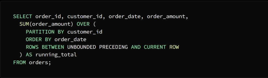
To calculate the current total for each individual customer, the SUM function must be applied to the order_amount column and divided by the customer_id column.
ORDER BY indicates that the rows are ordered according to the order dates in each section
Phrase:
ROWS BETWEEN UNBOUNDED PRECEDING AND CURRENT ROW
Indicates that the calculation is within the window between the rows at the beginning of the section up to the current row
The result of the query will come in the form of a table consisting of the same columns as the orders table, in addition to a column called run_total, which indicates the current total sales for each customer, and as we mentioned, arranged according to the dates of orders
* Common Table Phrases (CTEs)
CTEs allow you to get a set of results that can be used in SQL statements at a later time
For example: We have a table, let’s call it the Employees table, composed of the following columns:
employee_id, employee_name, department_id and salary
What is required is to calculate the average salary for each department, then search for employees with a higher salary than the average salary of the department to which they belong.
CTE can be used to perform two queries, the first to calculate the average salary of each department and the second to search for employees with higher salaries than the average salary of the department

We note here that the task has been divided into two phases to facilitate the query
The first stage is the salary calculation for each department
The second stage is to find the employees whose salary is higher than the average salary of the department to which they belong
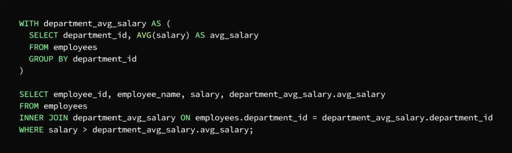
In the first query, CTE, called department_avg_salary, which is assigned to calculate the salary for each department, using the AVG function and the GROUP BY statement, which sorts the employees according to the department to which they belong.
As for the second query, CTE, called department_avg_salary, it is used as if it were a table, then it is joined to the employees table in the department_id column, and then the result is extracted by WHERE to finally get the employees with the highest salary from the average salary of the department they belong to.
* Aggregate functions
Aggregate functions can be defined briefly as functions whose task is to perform an arithmetic operation on a group of values to derive a result in the form of a single value, such as performing arithmetic operations in a table on several rows or columns in order to obtain a useful data summary.
In fact, the use of aggregate functions is a real advantage in the SQL language, as it makes queries in it more easy and accurate.
The functions SUM, AVG, MIN, MAX, and COUNT are the most used in SQL
To be clear: we have a sales table composed of the following columns
sale_id, product_id, sale_date, sale_amount, and region
It is required to calculate the total sales and the average sales for each product separately, and then determine the best-selling product in each region
This is done by following the following steps
We have to sort the sales by product and region, calculate the total and average sales, then discover the best-selling product in the region by using aggregate functions
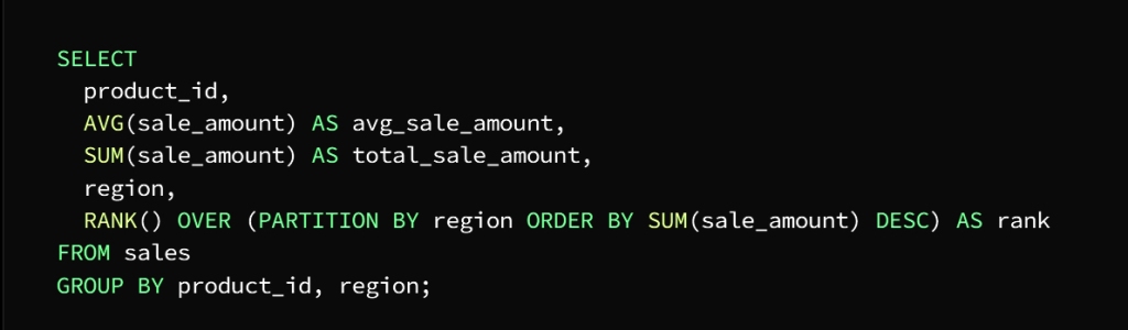
In this example, we use three aggregate functions AVG, SUM, and RANK
We will explain the task of each of them separately
AVG function calculates the average value of the product and the region
SUM function calculates the total value of each product and region using the GROUP BY statement
RANK function finds and explores the best-selling product in each region
To specify sorting by region, the OVER clause takes over this task
And to specify the column to divide the data (area) we use the PARTITION BY statement
As for getting the descending order of the sum of the value of each product in each region specified by the ORDER BY statement
The result of the query on a column shell is:
product_id, region, total_sale_amount, avg_sale_amount, and rank
So that the ranking column indicates the classification of each product in each region according to the total value of sale, so that the best-selling product in each region ranks first.
The uses of aggregate functions vary according to the tasks assigned to them. For example, you can calculate records, calculate maximum values, and other tasks.
* Pivot tables
They are tables that contain data extracted from large tables in order to analyze it easier, as it allows converting data from rows to columns to display the data in a more coordinated manner.
These tables are built using the PIVOT operator, whose task is to sort the data according to a specific column, and then show the results in the form of a formatted table.
To clarify
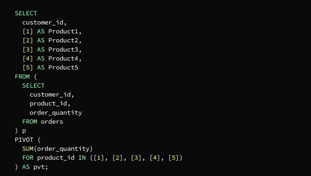
The PIVOT operator in the previous image is used to define the data axis by product_id plus columns per product and rows per customer
The SUM function calculates the total quantity of each product required by each customer
The p subquery extracts the necessary columns from the orders table
Then the PIVOT is run on the subquery in conjunction with the SUM function to find out the total quantity of each product ordered by each customer
The FOR statement is tasked with specifying the pivot column product_id in our example
The IN statement specifies target values ( [1], [2], [3], [4], [5] )
The pivot table appears as a result of a query for the total quantity ordered by each customer in the form of columns for each product and rows for each customer
* Subqueries
They are nested queries whose task is to retrieve data from one or more tables, and its results are used in the main query, and its function can be to sort and group data into one row or group of rows.
Subqueries such as SELECT, FROM, WHERE, HAVING are used within brackets in various places of the SQL statement.
To be clear: we have two tables
The first table is the employees table consisting of the following columns
employee_id, first_name, last_name, department_id
The second table is the payroll table and consists of the following columns
employee_id, salary, salary_date
It is required to know the highest paid employees in each department
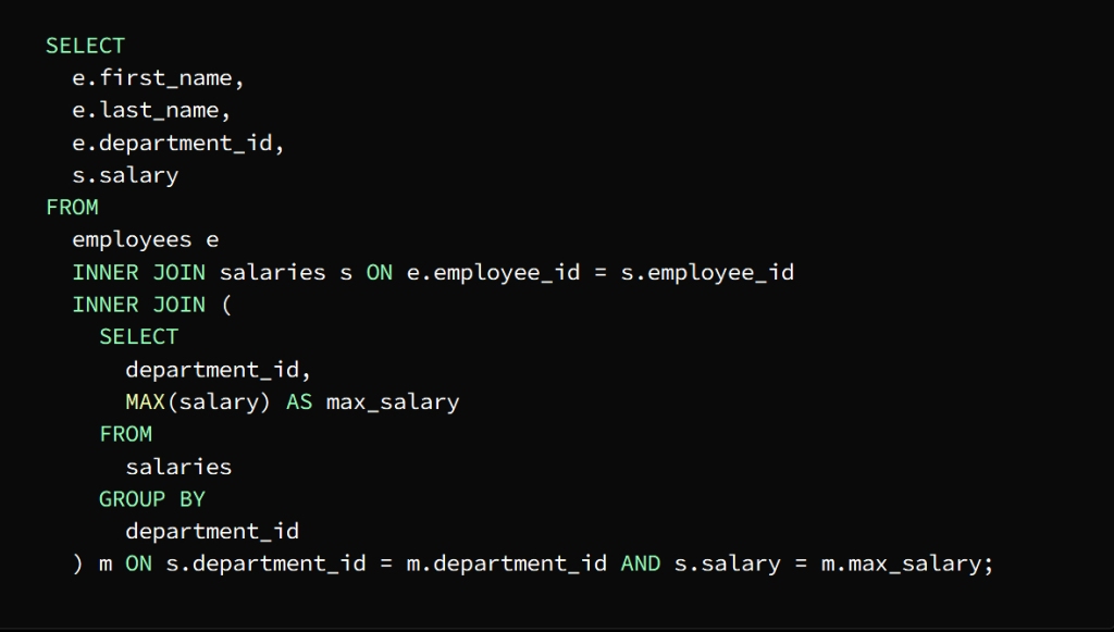
We can find the highest salary in each department using a subquery and then join the result to the Employees and Salaries tables to extract the names of the employees who earn that salary

After executing the subquery as a first step, a result set representing the highest salary in each department is returned, then the employee and salary tables are linked to the result of the subquery by means of the main query to extract the names of the highest paid employees in each department.
To demonstrate this join process, an INNER JOIN statement is used to join the Employee and Salary tables, using the employee_id column as the join key.
The subquery is joined to the main query using the department_id column
The salary column is then used to match the highest salary in each department
The result appears in the form of a table containing the names of the highest paid employees in each department along with the department ID and salary
* Cross Joins
Cross Joins are a type of join operation that returns the Cartesian product of two or more tables without using a join condition, but by combining rows from one table with rows from another table separately, then the result is a table consisting of the available combinations of rows from both tables
This operation is useful in certain circumstances, such as performing a calculation that requires all available value combinations from a set of tables, or generating test data, for example
For clarity we have two tables
The first table is the customers table and it consists of columns
customer_id, customer_name, and city
The second table is the orders table and it consists of columns
order_id, customer_id, and order_date
The requirement is to know the total number of orders for each customer in each city
This is done by creating a result set that includes each customer with each city and then joining the result to the orders table to extract the number of requests for each group
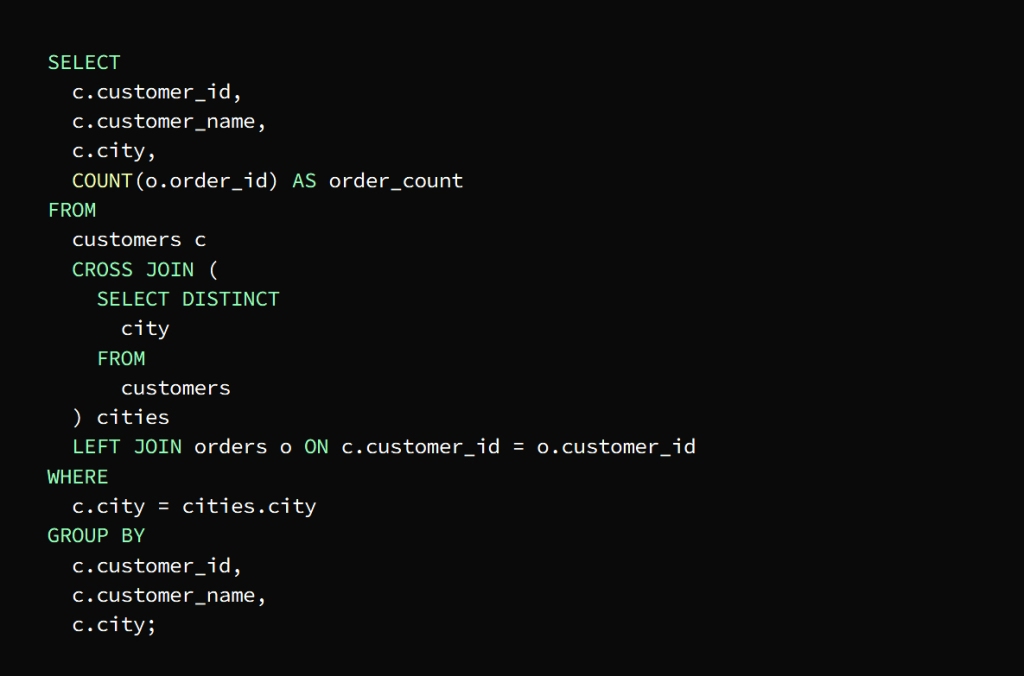
The previous image shows that a result set has been created that includes each customer with each city, and thus the query is Use cross join to return the result set that contains a group that includes the customer and the city
The main query then joins the result of the cross-join with the orders table
Important Notes :
Here left join should be used to keep clients visible in the result even if they did not place any order
In order to ensure that the result of the number of requests for each customer appears in his city, the WHERE clause is used to sort the results and get the rows that match the city in which the customer resides in the cross join
To group the result according to the customer’s ID, name, and city, we use the GROUP BY statement
To calculate the number of orders per customer in each city, we use the COUNT() function.
The result is finally shown in the form of a table containing the total number of orders for each customer in each city
* temporary tables
These tables are relied upon to store the intermediate results in memory or on disk and use them at the end of the work and then get rid of them automatically
Or this type of table is used to divide large and complex queries into smaller parts to make it easier to process
The CREATE TEMPORARY TABLE statement is used to create temporary tables
The SELECT, INSERT, UPDATE, DELETE commands are used to process these tables as if they were regular tables in order to reduce the amount of large and complex data to facilitate processing.
For clarity, we have a sales table consisting of the following columns
date, product, category, sales_amount
It is required to create a report showing the total sales for each category for each month over the past year
We can address this issue through the following actions
The first goal is to obtain the total sales for each category. This is done by creating a temporary table that includes a summary of sales data for each month, and then linking it to the sales table.
This is done by following these steps
Create the temporary table using the CREATE TEMPORARY TABLE statement
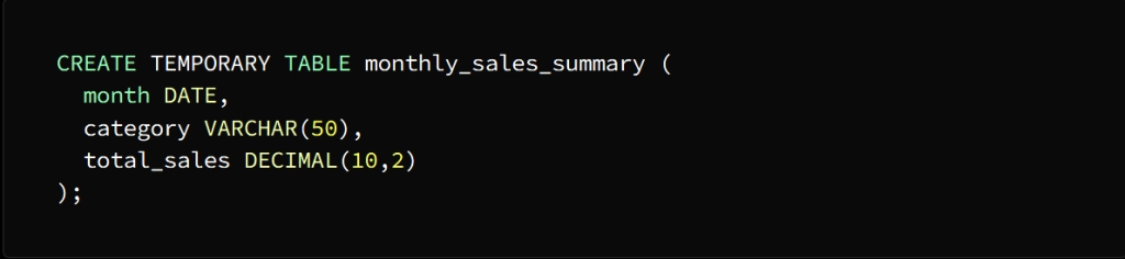
A temporary table named Monthly_sales_summary is created with three columns:
month, category, and total_sales
The month column is of type DATE
category column of type VARCHAR (50)
total_sales column of type DECIMAL(10,2)
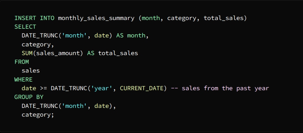
Using the INSERT INTO statement, we populate the temporary table with the shortened data

To separate the date column into the month level and group the sales data by month and category, we used the DATE_TRUNC function
Then we enter the result of this query into the month_sales_summary table, which now contains a summary of sales data for each month separately.
To get the total sales for each category we can join the temporary table with the sales table
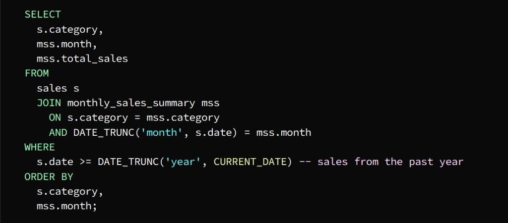
The Sales table is joined with the Monthly_sales_summary table in the columns designated for category and month
From the temporary table, the month, category, and total_sales columns can be selected
To get the required result, which is last year’s sales data, we use the WHERE phrase
To sort the result by category and month we use the ORDER BY statement
The result of the query appears in the form of a table containing the total sales for each category for each month of the previous year
* Materialized Views
The task of these insights is to improve the performance of frequently executed queries, which are various results that are previously stored in the form of actual tables and are called to the original tables without the need to perform operations in them
This process is used to improve the performance of complex queries through data storage and business intelligence applications, which contributes to shortening the time for preparing reports and raising the efficiency of dashboards

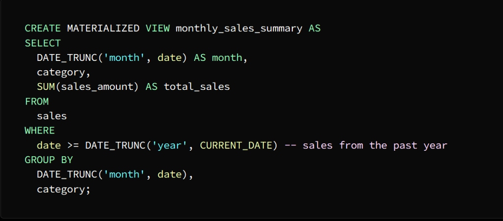
The image above shows that an actual offer named Monthly_sales_summary has been created
This presentation contains a summary of sales data for each category for each month
We use the SELECT statement to store the result in the actual view
Actual views are automatically updated when the underlying data changes although they are similar to tables stored on disk, and can also be updated manually using the
REFRESH MATERIALIZED VIEW
You can query the actual view once it is created just like any other table
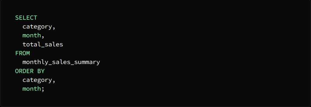
In the above image the category, month and total sales columns are selected from the actual view month_sales_summary and it sorts the result by category and month
As we mentioned earlier, with the actual view method, you can shorten a lot of the time it takes to run the query, as this method allows you to use pre-calculation and storage of summary data.
In conclusion:
Remember, my reader friend, that keeping abreast of developments and keeping pace with the accelerating technology is very important, and your knowledge of all new technologies and skills makes things easier for you and even increases your scientific level, whether in the field of programming and data analysis or in any other scientific field.
I hope that you have gained a great deal of interest, and please share this information and support the blog so that we can continue to provide everything new, and we are pleased to see your opinions on the comments, thank you.
SQL مجموعة تقنيات
متقدمة لا غنى عنها لكل عالِم بيانات

(SQL) لغة الاستعلام الهيكلية
هي لغة الاستعلام القياسية لقاعدة البيانات العلائقية، تمتاز هذه اللغة ببساطتها وسهولة فهمها، إلا أن الانتقال إلى مستوى متقدم في تحليل البيانات يتطلب إتقان التقنيات المتقدمة لهذه اللغة
وعندما نتحدث عن التقنيات المطلوب تعلمها للانتقال إلى مستوى متقدم فإننا نتحدث عن منظومة من الوظائف والميزات التي تتيح لك القيام بمهام معقدة على البيانات كالضم والتجميع والاستعلامات الفرعية ووظائف النافذة وغيرها من الوظائف الأخرى التي يمكنها التعامل مع البيانات الضخمة للحصول على نتائج فعالة ودقيقة
بعض الأمثلة الحية
المتقدمة SQL على استخدام تقنيات
وظائف النافذة *
من خلال هذه التقنية يمكنك تنفيذ عمليات حسابية عبر عدة صفوف مرتبطة بالصف المحدد
كأن يكون لدينا جدول طلبات يضم الأعمدة التالية
order_id, customer_id, order_date, order_amount
والمطلوب حساب المبيعات الإجمالي الحالي لكل عميل على حدة مرتبة حسب تاريخ الطلب
لتنفيذ هذه المهمة SUM بالإمكان الاستعانة بـ

ليتم حساب الإجمالي الحالي لكل عميل على حدى
SUM يجب تطبيق الدالة
order_amount على عمود
customer_id ويتم تقسيمها وفق العمود
ORDER BY تشير عبارة
إلى أن ترتيب الصفوف يتم وفق تواريخ الطلب في كل قسم
: تشير عبارة
ROWS BETWEEN UNBOUNDED PRECEDING AND CURRENT ROW
إلى أن الحساب يقع ضمن النافذة المحصورة بين الصفوف الواقعة في بداية القسم حتى الصف الحالي ستأتي نتيجة الاستعلام على شكل جدول مؤلف من نفس أعمدة جدول الطلبات
run_total مضافاً إليها عمود يسمى
والدال على المبيعات الإجمالية الحالية لكل عميل وكما ذكرنا مرتبة حسب تواريخ الطلبات
(CTEs) عبارات الجدول الشائعة*
CTEs تتيح لك
الحصول على مجموعة من النتائج التي يمكن الاستعانة بها
في وقت لاحق SQL في جمل
على سبيل المثال: لدينا جدول ولنطلق عليه اسم جدول الموظفين مؤلف من الأعمدة التالية
employee_id, employee_name, department_id, salary
والمطلوب حساب متوسط الراتب لكل قسم، ثم البحث عن الموظفين الأعلى راتباً من متوسط الراتب الخاص بالقسم الذي ينتمون إليه
لإجراء استعلامين CTE يمكن الاستعانة بـ
الأول لحساب متوسط الراتب كل قسم والثاني للبحث عن الموظفين الأعلى راتباً من متوسط راتب القسم
نلاحظ هنا أنه تم تقسيم المهمة إلى مرحلتين لتسهيل الاستعلام
مرحلة أولى وهي حساب الراتب لكل قسم
مرحلة ثانية إيجاد الموظفين الأعلى راتباً من متوسط راتب القسم الذي ينتمون إليه
CTE ففي الاستعلام الأول
department_avg_salary والمسمى
المخصص لحساب الراتب لكل قسم وذلك باستخدام
GROUP BY وعبارة AVG دالة
التي تقوم بفرز الموظفين كلٌ حسب القسم الذي ينتمي إليه
CTE أما الاستعلام الثاني
department_avg_salary المسمى
فيستخدم كما لو كان جدولاً ثم يتم
department_id ضمه إلى جدول الموظفين في العمود
WHERE ثم يتم استخلاص النتيجة بواسطة
لنحصل في النهاية على الموظفين الأعلى راتباً من متوسط الراتب الخاص بالقسم الذي ينتمون إليه
الدالات التجميعية *
يمكن تعريف الدالات التجميعية بشكل مختصر على أنها وظائف مهمتها إجراء عملية حسابية على مجموعة من القيم لاستخلاص نتيجة على شكل قيمة واحدة كإجراء عمليات حسابية في جدول على عدة صفوف أو أعمدة بغية الحصول على خلاصة بيانات مفيدة
وفي الحقيقة يعتبر استخدام الدالات التجميعية
SQL مكسباً حقيقياً في لغة
إذ تجعل الاستعلامات فيها أكثر سهولة ودقة
وتعتبر الدالات
SUM, AVG, MIN, MAX, COUNT
SQL هي الأكثر استخداماً في
وللتوضيح: لدينا جدول مبيعات مؤلف من الأعمدة التالية
sale_id, product_id, sale_date, sale_amount, region
والمطلوب حساب المبيعات الإجمالية ومتوسط المبيعات الخاصة بكل منتج على حدة ثم تحديد المنتج الأكثر مبيعاً في كل منطقة
يتم ذلك من خلال اتباع الخطوات التالية
علينا فرز المبيعات حسب المنتج والمنطقة وحساب إجمالي ومتوسط المبيعات ثم اكتشاف المنتج الأكثر مبيعاً في المنطقة وذلك عن طريق الاستعانة بالدالات التجميعية

استخدمنا في هذا المثال
AVG, SUM, RANK ثلاث دالات تجميعية
وسنبين مهمة كل واحدة منها على حدة
AVG الدالة
مهمتها حساب متوسط قيمة المنتج والمنطقة
SUM الدالة
مهمتها حساب القيمة الإجمالية لكل منتج والمنطقة
GROUP BY باستخدام عبارة
RANK الدالة
مهمتها استكشاف المنتج الأكثر مبيعاً في كل منطقة
ولتحديد الفرز وفق كل منطقة
هذه المهمة OVER تتولى عبارة
ولتحديد العمود لتقسيم البيانات (المنطقة)
PARTITION BY نستخدم عبارة
أما للحصول على الترتيب التنازلي لمجموع قيمة كل منتج في
ORDER BY كل منطقة تحدده عبارة
: تأتي نتيجة الاستعلام على شكل أعمدة هي
product_id, region, total_sale_amount, avg_sale_amount, rank
بحيث يدل عمود الترتيب على تصنيف كل منتج في كل منطقة وفق القيمة الإجمالية للبيع بحيث يحصل المنتج الأكثر مبيعاً في كل منطقة على المرتبة الأولى
تتنوع استخدامات الدالات التجميعية حسب المهام الموكلة إليها فيمكنك مثلاً حساب السجلات وحساب الحد الأقصى للقيم وغيرها من المهام الأخرى
الجداول المحورية *
وهي جداول تحوي بيانات مستخلصة من جداول كبيرة بغية تحليلها بشكل أسهل بحيث تتيح تحويل البيانات من الصفوف إلى الأعمدة لعرض البيانات بشكل أكثر تنسيقاً
يتم بناء هذه الجداول
PIVOT بالاستعانة بعامل التشغيل
والذي مهمته فرز البيانات وفق عمود معين ثم إظهار النتائج على شكل جدول منسق
للتوضيح

PIVOT استُخدِمَ عامل التشغيل
في الصورة السابقة لتحديد محور البيانات
product_id حسب معرف المنتج
بالإضافة إلى أعمدة لكل منتج وصفوف لكل عميل
SUM يأتي دور الدالة
لتقوم بحساب الكمية الإجمالية لكل منتج مطلوب من قبل كل عميل
pأما الاستعلام الفرعي
يتولى مهمة استخراج الأعمدة الضرورية من جدول الطلبات
PIVOT ثم يتم تشغيل
على الاستعلام الفرعي بالتعاون
SUM مع الدالة
لمعرفة الكمية الإجمالية لكل منتج يتم طلبه من قبل كل عميل
FOR أما عبارة
product_id فمهمتها تحديد العمود المحوري
في مثالنا هذا
IN أما عبارة
تحدد القيم المستهدفة ( [1]، [2]، [3]، [4]، [5] )
يظهر الجدول المحوري كنتيجة للاستعلام عن الكمية الإجمالية التي طلبها كل عميل على شكل أعمدة لكل منتج وصفوف لكل عميل
الاستعلامات الفرعية *
وهي استعلامات متداخلة مهمتها استعادة بيانات من جدول واحد أو أكثر ونتائجها تستخدم في الاستعلام الرئيسي كما ويمكن أن تكون وظيفتها فرز البيانات وتجميعها في صف واحد أو مجموعة صفوف تستخدم الاستعلامات الفرعية مثل
SELECT, FROM, WHERE, HAVING
SQL ضمن أقواس في أماكن متعددة من عبارة
وللتوضيح: لدينا جدولين
الجدول الأول هو جدول الموظفين يتألف من الأعمدة التالية
employee_id, first_name, last_name, department_id
الجدول الثاني هو جدول الرواتب ويتألف من الأعمدة التالية
employee_id, salary, salary_date
والمطلوب معرفة الموظفين الأعلى راتباً في كل قسم
يمكننا إيجاد الراتب الأعلى في كل قسم باستخدام استعلام فرعي ثم ضم النتيجة إلى جدولَي الموظفين والرواتب لاستخلاص أسماء الموظفين الذين يتقاضون هذا الراتب
بعد تنفيذ الاستعلام الفرعي كخطوة أولى يتم إرجاع مجموعة نتائج تمثل الراتب الأعلى في كل قسم ثم يتم ربط جداول الموظفين والرواتب بنتيجة الاستعلام الفرعي بواسطة الاستعلام الرئيسي لاستخراج أسماء الموظفين الأعلى راتباً في كل قسم
ولشرح عملية الانضمام هذه
INNER JOIN تستخدم عبارة
للانضمام إلى جداول الموظفين والرواتب وذلك باستخدام
كمفتاح الانضمام employee_id العمود معرف الموظف
ويتم ربط الاستعلام الفرعي بالاستعلام الرئيسي
department_id باستخدام العمود معرف القسم
salary ثم يتم استخدام عمود الراتب
لمطابقة الراتب الأعلى في كل قسم
فتظهر النتيجة على شكل جدول يحوي أسماء الموظفين الأعلى راتباً في كل قسم بجانب معرف القسم والراتب
Cross Joins
Cross Joins عمليات الانضمام المتقاطعة
هي أحد أنواع عمليات الربط التي تعيد المنتج الديكارتي لجدولين أو أكثر دون استخدام شرط ربط بل بتجميع صفوف من جدول مع صفوف من جدول آخر كل على حدة ثم تكون النتيجة جدول يتألف من مجموعات الصفوف المتاحة من كلا الجدولين
تفيد هذه العملية في ظروف معينة كإجراء عملية حسابية تتطلب كل مجموعات القيمة المتاحة من مجموعة جداول أو إنشاء بيانات الاختبار مثلاً
للتوضيح لدينا جدولان
وهو يتألف من الأعمدة customers الجدول الأول هو جدول العملاء
customer_id, customer_name, city
وهو يتألف من الأعمدة orders الجدول الثاني هو جدول الطلبات
order_id, customer_id, order_date
المطلوب هو معرفة عدد الإجمالي لطلبات كل عميل في كل مدينة
يتم ذلك بإنشاء مجموعة نتائج تضم كل عميل مع كل مدينة ثم ضم النتيجة إلى جدول الطلبات لاستخراج عدد طلبات كل مجموعة

توضح الصورة السابقة أنه تم إنشاء مجموعة نتائج تضم كل عميل مع كل مدينة
cross join وبهذا يكون الاستعلام استخدم
لتعود مجموعة النتائج التي تحتوي مجموعة تضم العميل والمدينة
ثم ينضم الاستعلام الرئيسي إلى نتيجة الضم التبادلي مع جدول الطلبات
:ملاحظات هامة
left join هنا يجب استخدام
للمحافظة على ظهور العملاء في النتيجة حتى لو لم يقوموا بتقديم أي طلب
ولضمان ظهور نتيجة عدد طلبات كل عميل في مدينته
WHERE تستخدم عبارة
لفرز النتائج والحصول على الصفوف التي تطابق المدينة
cross join التي يقيم فيها العميل في
لتجميع النتيجة وفق معرف العميل واسمه ومدينته
GROUP BY نستخدم عبارة
ولحساب عدد طلبات كل عميل في كل مدينة
COUNT () نستخدم الدالة
تظهر النتيجة في النهاية على شكل جدول يحتوي العدد الإجمالي لطلبات كل عميل في كل مدينة
جداول مؤقتة *
يتم الاعتماد على هذه الجداول لتخزين النتائج الوسيطة في الذاكرة أو على القرص واستخدامها في نهاية العمل ثم التخلص منها تلقائياً
أو يستخدم هذا النوع من الجداول لتقسيم الاستعلامات الكبيرة والشائكة إلى أجزاء أصغر لتسهيل معالجتها
CREATE TEMPORARY TABLE تستخدم عبارة
لإنشاء الجداول المؤقتة
SELECT, INSERT, UPDATE, DELETE وتستخدم الأوامر
لمعالجة تلك الجداول كأنها جداول عادية بغية تقليل كمية البيانات الكبيرة والمعقدة لتسهيل معالجتها
وللتوضيح لدينا جدول مبيعات يتألف من الأعمدة التالية
date, product, category, sales_amount
والمطلوب إنشاء تقرير يبين المبيعات الإجمالية لكل فئة لكل شهر على خلال العام الفائت
يمكننا معالجة هذا الموضوع من خلال الإجراءات التالية
الهدف الأول هو الحصول على إجمالي المبيعات لكل فئة ويتم ذلك بإنشاء جدول مؤقت يشمل ملخص لبيانات المبيعات عن كل شهر ثم ربطه بجدول المبيعات
ويتم ذلك باتباع الخطوات التالية
:إنشاء الجدول المؤقت
وذلك باستخدام عبارة
CREATE TEMPORARY TABLE

Monthly_sales_summary فينشأ جدول مؤقت يسمى
يتألف من ثلاثة أعمدة
month, category, total_sales
DATEمن النوع month عمود الشهر
VARCHAR (50) من نوع category عمود الفئة
total_sales عمود إجمالي المبيعات
DECIMAL (10،2) من نوع
INSERT INTO وباستخدام عبارة
نقوم بتعبئة الجدول المؤقت بالبيانات المختصرة
لفصل عمود التاريخ إلى المستوى الشهر وتجميع بيانات المبيعات وفق الشهر والفئة
DATE_TRUNC استخدمنا الدالة
ثم نقوم بإدخال نتيجة هذا الاستعلام
month_sales_summary في جدول
الذي أصبح يحوي ملخص لبيانات مبيعات كل شهر على حدة وللحصول على إجمالي مبيعات كل فئة يمكننا الانضمام إلى الجدول المؤقت مع جدول المبيعات

يتم الانضمام إلى جدول المبيعات
Monthly_sales_summary مع جدول
في الأعمدة المخصصة للفئة والشهر
ومن الجدول المؤقت يمكن تحديد أعمدة
month, category, total_sales
ولنحصل على النتيجة المطلوبة وهي بيانات مبيعات العام الماضي
WHERE نستخدم عبارة
ولفرز النتيجة حسب الفئة والشهر
ORDER BY نستخدم عبارة
تظهر نتيجة الاستعلام على شكل جدول يحوي إجمالي المبيعات لكل فئة عن كل شهر من العام الفائت
الرؤى الفعلية *
مهمة هذه الرؤى تحسين أداء الاستعلامات التي يتم تنفيذها بشكل متكرر وهي عبارة عن نتائج متنوعة مخزنة مسبقاً على شكل جداول فعلية ويتم استدعاؤها إلى الجداول الأصلية دون الحاجة إلى إجراء العمليات فيها
يستفاد من هذه العملية في تحسين أداء الاستعلامات المعقدة من خلال تخزين البيانات وتطبيقات ذكاء الأعمال مما يسهم في اختصار الوقت بالنسبة لإعداد التقارير ورفع كفاءة لوحات المعلومات
توضح الصورة أعلاه أنه تم إنشاء
Monthly_sales_summary عرض فعلي اسمه
هذا العرض يحوي ملخص لبيانات المبيعات لكل فئة عن كل شهر
SELECT نستخدم عبارة
لتخزين النتيجة في الرؤية الفعلية
يتم تحديث طرق العرض الفعلية تلقائياً عندما تتغير البيانات الأساسية على الرغم من أنها تشبه الجداول من حيث تخزينها على القرص، كما ويمكن تحديثها يدوياً باستخدام عبارة
REFRESH MATERIALIZED VIEW
يمكنك الاستعلام عن العرض الفعلي بمجرد إنشائه كأي جدول آخر

في الصورة أعلاه يتم تحديد أعمدة الفئة والشهر وإجمالي المبيعات
month_sales_summary من طريقة العرض الفعلية
ويقوم بفرز النتيجة وفق الفئة والشهر
كما ذكرنا سابقاً بطريقة العرض الفعلي يمكنك اختصار الكثير من الوقت الذي يستغرقه تشغيل الاستعلام إذ أن هذه الطريقة تتيح لك استخدام الحساب المسبق لبيانات الملخص وتخزينها
:ختاماً
تذكر صديقي القارئ أن مواكبة التطورات والسير في ركب التكنولوجيا المتسارعة أمر غاية في الأهمية ومعرفتك بكل ما جديد من تقنيات ومهارات يسهل عليك كثيراً من الأمور بل ويزيد من مستواك العلمي سواء في مجال البرمجة وتحليل البيانات أو في أي مجال علمي آخر
أتمنى أن تكونوا قد حصلتم على قسط كبير من الفائدة ونرجو مشاركة هذه المعلومات ودعم المدونة لنستمر في تقديم كل ما هو جديد ويسعدنا مشاهدة آرائكم على التعليقات وشكراً
