


The Excel program is one of the programs that has features and characteristics that help the user to analyze data easily, and due to the multiple formulas and functions it provides that are capable of carrying out a set of operations, from which we will discuss in our article these functions of calculations, character and date text tasks, and a set of other research tasks
1. CONCATENATE
This formula is considered one of the most effective formulas in analyzing data, despite its ease and simplicity of working with it. Its task is to use dates, texts, numbers, and different data present in several cells and merge them into one cell.
SYNTAX = CONCATENATE (text1, text2, [text3], …)

Concatenate multiple cell values
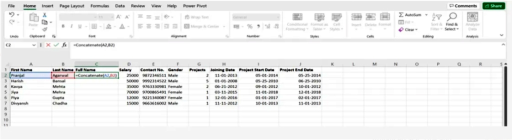
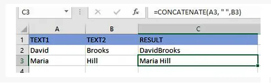
The simple CONCATENATE formula for the values of two cells A2 and B2 is as follows:
= CONCATENATE (A2, B2)
The values will be combined without using any delimiter, and to separate the values with a space we use “ ”
=CONCATENATE(A3, “ “, B3)

Connect a string of texts and the computed value
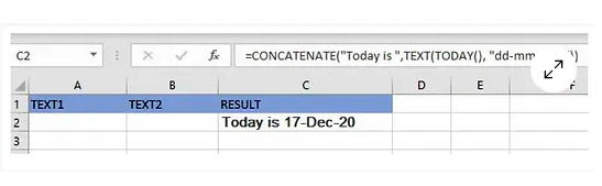
You can also bind a string and a computed value to the formula as in the example of restoring the current date
=CONCATENATE(“Today is ”, TEXT(TODAY(), “dd-mmm-yy”))
You can verify that the results provided by the CONCATENATE function are correct by doing the following:
In all cases, the result of the CONCATENATE function is a text string, even if all the source values are numbers
Make sure there is a text argument in the CONCATENATE function to ensure that it works
You have to pay close attention to the validity of the text argument in order for the CONCATENATE function to work correctly, otherwise the formula will return the error #VALUE! This is because the arguments are not valid
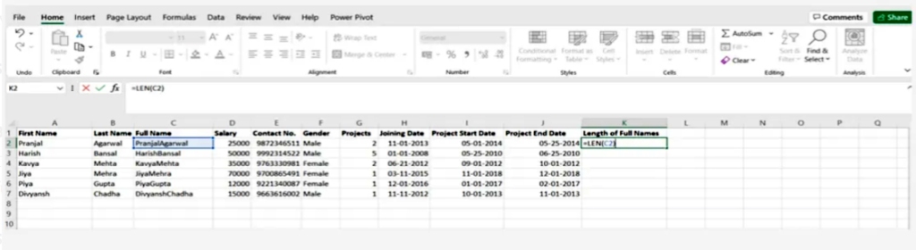
2.Len()
This function is used to know the number of characters in one cell, or when dealing with text that contains a limited number of characters, or to know the difference between the numbers of a group of products
SYNTAX = LEN (text)

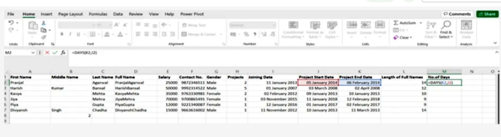
3.Days()
This function is used to calculate the number of days between two dates
SYNTAX = DAYS (end_date, start_date)

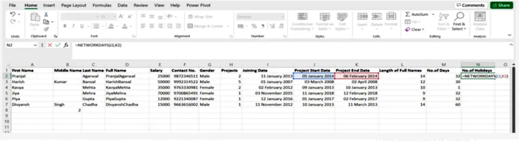
4.Networkdays
It is considered to be a function of date and time in Excel and is often used by finance and accounting departments to exclude the number of weekends to determine the wages of employees based on the calculation of actual working days for them or the calculation of the total number of working days for a specific project
SYNTAX = NETWORKDAYS (start_date, end_date, [holidays])

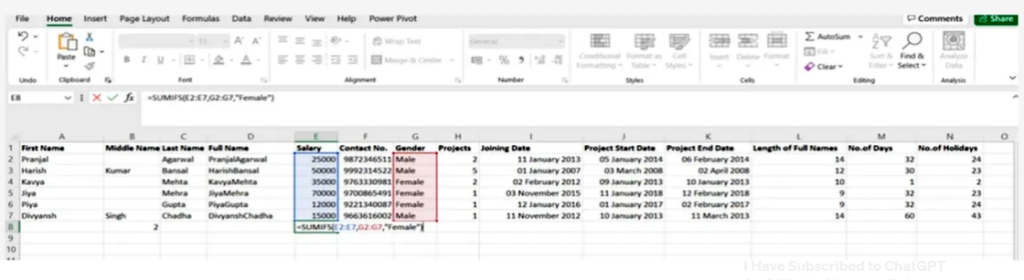
5.Sumifs()
It is one of the most common formulas in Excel and is considered one of the most important functions for data analysts =SUMIFS. =SUM, especially for conducting data collection under sample conditions
SYNTAX = SUMIFS (sum_range, range1, criteria1, [range2], [criteria2], …)

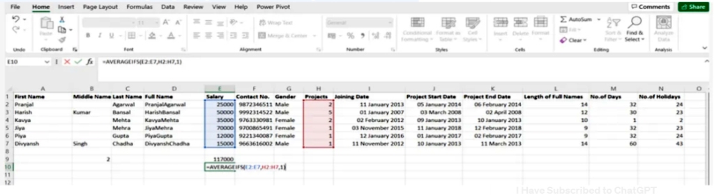
6. Averageifs()
This task allows the average to be extracted from one or more parameters
SYNTAX = AVERAGEIFS (avg_rng, range1, criteria1, [range2], [criteria2], …)

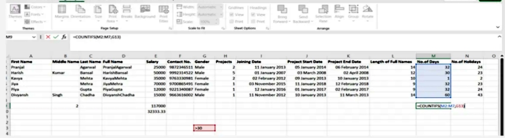
7. Countsifs()
It is an important tool in data analysis and it is similar to SUMIFS. In most functions it counts the number of values that satisfy certain conditions but it doesn’t need a summation range
SYNTAX = COUNTIFS (range, criteria)

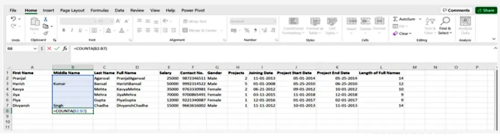
8.Count()
Its job is to determine whether a cell is empty or not by discovering gaps in the data set without you, as a data analyst, having to restructure it.
SYNTAX = COUNTA (value1, [value2], …)

9. Vlookup()
This shortcut stands for Vertically searching for a value in the leftmost column of the table so that you can return a value in the same row of the column you specify
SYNTAX = VLOOKUP (lookup_value, table_array, column_index_num, [range_lookup])
We will explain the arguments to the VLOOKUP function
– lookup_value : is the value to look up in the first column of the table
table – : indicates the table from which the value is to be retrieved
-col_index: returns the column in the table from the value
range_lookup – :
Optional: TRUE = approximate match
Default: FALSE = exact match
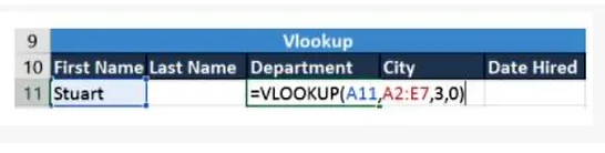
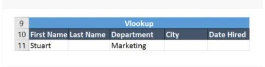
The following table will explain the use of VLOOKUP
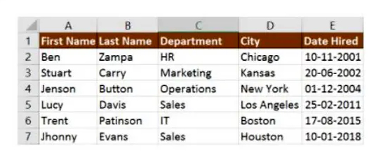
Cell A11 contains the lookup value
A2:E7 is the table array
3 is the column index with the information for the sections
0 is the search for the range

If you press the Enter key, it will return “Marketing”, which indicates that Stuart works in the marketing department

10. Lookup()
In it, “horizontal” is represented by the letter H, and it searches for one or more values in the top row of the table, then it retrieves a value from a row you specify in the table or row from the same column if this tool makes things easier, for example when the values you use are in the rows The first one from the spreadsheet and you need to look at a certain number of rows, this tool will do the trick
SYNTAX = HLOOKUP (lookup_value, table_array, row_index, [range_lookup])
Let’s learn about Hlookup’s arguments
Lookup_Value denotes the attached value
table — the table from which you need to retrieve data
ROW_INDEX which is the row number to restore the data
Range_lookup for exact and approximate matching, and that is determined by specifying the validity of the default value, so the match is approximate
In our next example, we’ll search for the city Jenson is from using Hlookup.
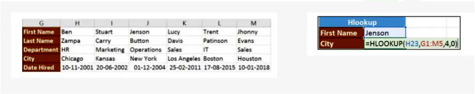
The search value shown in H23 is Jenson
G1: M5 is the table array
4 is the row index number
0 is for an approximate match
Pressing enter will take you back to New York.

at the end
We conclude from the above how effective Excel is in analyzing data. By learning its formulas and functions, you can make work easier for you and thus save a lot of time and effort.
عشرة وظائف لإكسل في تحليل البيانات

يعتبر برنامج إكسل من البرامج التي تتمتع بميزات وخصائص تعين المستخدم على تحليل البيانات بسهولة ونظراً لما يوفره من صيغ ووظائف متعددة قادرة على تنفيذ مجوعة عمليات سنتناول منها في مقالنا هذه وظائف العمليات الحسابية ومهام نصوص الأحرف والتاريخ ومجموعة أخرى من مهام البحث
CONCATENATE 1
تعتبر هذه الصيغة من الصيغ الأكثر فاعلية في تحليل البيانات رغم سهولتها وبساطة العمل بها وهي مهمتها استخدام التواريخ والنصوص والأرقام وبيانات مختلفة موجودة في عدة خلايا ودمجها في خلية واحدة
SYNTAX = CONCATENATE (text1, text2, [text3], …)
تسلسل قيم خلايا متعددة
CONCATENATE صيغة
A2 و B2 البسيطة لقيم خليتين
هي كما يلي
= CONCATENATE (A2، B2)
“ “سيتم دمج القيم بدون استخدام أي محدد ، ولفصم القيم بمسافة نستخدم
=CONCATENATE(A3, “ “, B3)
ربط سلسلة من النصوص والقيمة المحسوبة
كما ويمكنك ربط سلسلة نصية وقيمة محسوبة بالصيغة كما في المثال الموضح عن استعادة التاريخ الحالي
=CONCATENATE(“Today is “, TEXT(TODAY(), “dd-mmm-yy”))

ويمكنك التأكد من صحة النتائج التي تقدمها
CONCATENATE الدالة
من خلال اتباع ما يلي
في جميع الأحوال تكون نتيجة *
CONCATENATE الدالة
عبارة عن سلسلة نصية وإن كانت جميع قيم المصدر أرقاماً
احرص على وجود وسيطة نصية في *
CONCATENATE دالة
لضمان عملها
وعليك أن تنتبه جيداً من صحة الوسيطة النصية لكي تعمل *
CONCATENATE الدالة
بشكل صحيح وإلا فالصيغة
#VALUE! سترجع لك الخطأ
وهذا سببه أن الوسيطات غير صالحة
Len() 2.
تستخدم هذه الدالة لمعرفة عدد الأحرف في الخلية الواحدة ، أو عند التعامل مع نص يحوي عدد محدود من الأحرف أو معرفة الاختلاف بين أرقام مجموعة من المنتجات
SYNTAX = LEN (text)
Days() 3.
تستخدم هذه الدالة لحساب عدد الأيام الواقعة بين تاريخين
SYNTAX =DAYS (end_date, start_date)
Networkdays4.
وهي تعتبر أنها دالة التاريخ والوقت في إكسل وتستخدم غالباً من قبل أقسام المالية والمحاسبة لاستبعاد عدد عطلات نهاية الأسبوع لتحديد أجور الموظفين بناءً على حساب أيام العمل الفعلية لهم أو حساب عدد كامل أيام العمل لمشروع معين
SYNTAX = NETWORKDAYS (start_date, end_date, [holidays])
Sumifs() 5.
وهي من الصيغ المتداولة بكثرة في إكسل وتعتبر من أهم الوظائف بالنسبة لمحللي البيانات
=SUMIFS. =SUM
وخصوصاً لإجراء عملية جمع للبيانات وفق شروط معينة
SYNTAX = SUMIFS (sum_range, range1, criteria1, [range2], [criteria2], …)
Averageifs() 6.
تتيح هذه المهمة استخلاص المتوسط من معلمة واحدة أو أكثر
SYNTAX = AVERAGEIFS (avg_rng, range1, criteria1, [range2], [criteria2], …)
Countsifs() 7.
من الأدوات المهمة في تحليل البيانات
SUMIFS. وهي تتشابه مع
في معظم الوظائف فهي تقوم بحساب عدد القيم التي تحقق شروط معينة إلا أنها لا تحتاج إلى نطاق جمع
SYNTAX = COUNTIFS (range, criteria)
8. Counta()
مهمتها هي أن تحدد هل الخلية فارغة أم لا من خلال اكتشاف الفجوات الموجودة في مجموعة البيانات دون أن تضطر كمحلل بيانات إلى إعادة هيكلتها
SYNTAX = COUNTA (value1, [value2], …)
9. Vlookup()
يدل هذا الاختصار على البحث الشاقولي عن قيمة ما في العمود الكائن في أقصى يسار الجدول ليتسنى لك إرجاع قيمة في نفس الصف من العمود الذي تحدده
SYNTAX = VLOOKUP (lookup_value, table_array, column_index_num, [range_lookup])
VLOOKUP وسنقوم بشرح الوسيطات للدالة
lookup_value
هي القيمة التي عليك البحث عنها في العمود الأول من الجدول
table
يدل على الجدول التي يتم استرداد القيمة منه
col_index
يتيح استعادة العمود الموجود في الجدول من القيمة
range_lookup
اختياري : TRUE = approximate match
افتراضي : FALSE = exact match
VLOOKUP وسيوضح الجدول التالي استخدام

lookup تحوي قيمة A11 الخلية
هي صفوف الجدول A2: E7
رقم 3 هو فهرس العمود مع المعلومات الخاصة بالأقسام
رقم 0 هو البحث عن النطاق
Enter وفي حال الضغط على مفتاح
فسيعيد “التسويق” وهذه دلالة على أن
يعمل في قسم التسويق Stuart
10. Hlookup()
“وفيه يمثل “الأفقي
H بالحرف
وهو يبحث عن قيمة واحدة أو أكثر في الصف العلوي من الجدول، ثم يقوم باستعادة قيمة من صف تحدده في الجدول أو الصف من نفس العمود إذا تقوم هذه الأداة بتسهيل الأمور أكثر فمثلاً عند تكون القيم التي تستخدمها موجودة في الصفوف الأولى من جدول البيانات واحتجت إلى أن تتطلع على عدد صفوف معين فهذه الأداة تفي بالغرض
SYNTAX = HLOOKUP (lookup_value, table_array, row_index, [range_lookup])
Hlookup لنتعرف على وسيطات
Lookup_Value
يدل على القيمة المرفقة
table —
وهو الجدول الذي عليك استعادة البيانات منه
ROW_INDEX
وهو رقم الصف لاستعادة البيانات
Range_lookup
للمطابقة الدقيقة والتقريبية وذلك يتحدد بتحديد صحة القيمة الافتراضية فبصحتها يكون التطابق تقريبي
في مثالنا التالي سنقوم بالبحث عن المدينة
Jenson التي ينتمي إليها
Hlookup. باستخدام

Jenson وهي H23 تظهر قيمة البحث في
هي صفوف الجدول G1: M5
رقم 4 فهرس الصف
رقم 0 اختبار تقريبي
Enter وبالضغط على
“سيعيدك إلى ” نيويورك

وفي الختام
نستخلص مما سبق مدى فاعلية إكسل في تحليل البيانات فبتعلمك صيغه ووظائفه يمكنك تسهيل العمل عليك وبالتالي توفر الكثير من الوقت والجهد

Thanks for your marvelous posting! I really enjoyed reading it, you can be a great author.I will make certain to bookmark your blog and will eventually come back at some point. I want to encourage that you continue your great writing, have a nice weekend!
LikeLiked by 1 person
Thanks for posting. I really enjoyed reading it, especially because it addressed my problem. It helped me a lot and I hope it will help others too.
LikeLike